R Visualization: Introduction to Distributions

Introduction to Distributions

• A distribution is a function or description that shows the possible values of a variable and how often those values occur.
• For categorical variables, the distribution describes the proportions of each category.
• A frequency table is the simplest way to show a categorical distribution. Use prop.table() to convert a table of counts to a frequency table. Barplots display the distribution of categorical variables and are a way to visualize the information in frequency tables.
• For continuous numerical data, reporting the frequency of each unique entry is not an effective summary as many or most values are unique. Instead, a distribution function is required.
• The cumulative distribution function (CDF) is a function that reports the proportion of data below a value a for all values of a: F(a)=Pr(x≤a).
• The proportion of observations between any two values a and b can be computed from the CDF as F(b)−F(a). A histogram divides data into non-overlapping bins of the same size and plots the counts of number of values that fall in that interval.

Code: Distribution of Heights Example

# load the dataset
library(dslabs)
data(heights)

# make a table of category proportions
prop.table(table(heights$sex))

Cumulative Distribution Function

Every continuous distribution has a cumulative distribution function (CDF). The CDF defines the proportion of the data below a given value a for all values of a:
F(a)=Pr(x≤a)
Any continuous dataset has a CDF, not only normal distributions. For example, the male heights data we used in the previous section has this CDF:

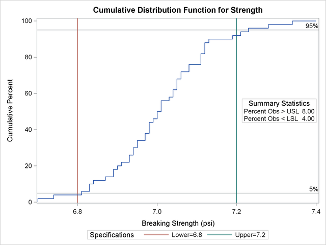
As defined above, this plot of the CDF for male heights has height values a on the x-axis and the proportion of students with heights of that value or lower (F_(a)_) on the y-axis.
The CDF is essential for calculating probabilities related to continuous data. In a continuous dataset, the probability of a specific exact value is not informative because most entries are unique. For example, in the student heights data, only one individual reported a height of 68.8976377952726 inches, but many students rounded similar heights to 69 inches. If we computed exact value probabilities, we would find that being exactly 69 inches is much more likely than being a non-integer exact height, which does not match our understanding that height is continuous. We can instead use the CDF to obtain a useful summary, such as the probability that a student is between 68.5 and 69.5 inches.
For datasets that are not normal, the CDF can be calculated manually by defining a function to compute the probability above. This function can then be applied to a range of values across the range of the dataset to calculate a CDF. Given a dataset my_data, the CDF can be calculated and plotted like this:

a <- seq(min(my_data), max(my_data), length = 100)    # define range of values spanning the dataset
cdf_function <- function(x) {    # computes prob. for a single value
    mean(my_data <= x)
}
cdf_values <- sapply(a, cdf_function)
plot(a, cdf_values)

The CDF defines that proportion of data below a cutoff _a_. To define the proportion of values above _a_, we compute:
**1−F(a)**
To define the proportion of values between _a_ and _b_, we compute:
**F(b)−F(a)**
Note that the CDF can help compute probabilities. The probability of observing a randomly chosen value between _a_ and _b_ is equal to the proportion of values between _a_ and _b_, which we compute with the CDF.

Smooth Density Plot

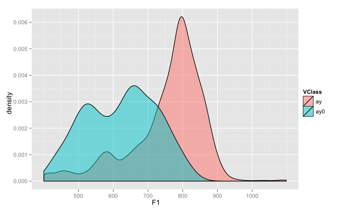
• Smooth density plots can be thought of as histograms where the bin width is extremely or infinitely small. The smoothing function makes estimates of the true continuous trend of the data given the available sample of data points.
• The degree of smoothness can be controlled by an argument in the plotting function.
• While the histogram is an assumption-free summary, the smooth density plot is shaped by assumptions and choices you make as a data analyst.
• The y-axis is scaled so that the area under the density curve sums to 1. This means that interpreting values on the y-axis is not straightforward. To determine the proportion of data in between two values, compute the area under the smooth density curve in the region between those values.
• An advantage of smooth densities over histograms is that densities are easier to compare visually.

Normal Distribution

• The normal distribution:
  • Is centered around one value, the mean
  • Is symmetric around the mean
  • Is defined completely by its mean (μ) and standard deviation ( σ )
  • Always has the same proportion of observations within a given distance of the mean (for example, 95% within 2 σ)
• The standard deviation is the average distance between a value and the mean value.
• Calculate the mean using the mean() function.
• Calculate the standard deviation using the sd() function or manually.
• Standard units describe how many standard deviations a value is away from the mean. The z-score, or number of standard deviations an observation x is away from the mean μ:
  Z = (x-μ)/σ

* Compute standard units with the scale() function. * **Important:** to calculate the proportion of values that meet a certain condition, use the **mean()** function on a logical vector. Because TRUE is converted to 1 and FALSE is converted to 0, taking the mean of this vector yields the proportion of TRUE.

Code: Normal Distributions

# define x as vector of male heights
library(tidyverse)
library(dslabs)
data(heights)
index <- heights$sex=="Male"
x <- heights$height[index]

# calculate the mean and standard deviation manually
average <- sum(x)/length(x)
SD <- sqrt(sum((x - average)^2)/length(x))

# built-in mean and sd functions - note that the audio and printed values disagree
average <- mean(x)
SD <- sd(x)
c(average = average, SD = SD)

# calculate standard units
z <- scale(x)

# calculate proportion of values within 2 SD of mean
mean(abs(z) < 2)

Normal CDF and pnorm

• The normal distribution has a mathematically defined CDF which can be computed in R with the function pnorm().
• pnorm(a, avg, s) gives the value of the cumulative distribution function F(a) for the normal distribution defined by average avg and standard deviation s.
• We say that a random quantity is normally distributed with average avg and standard deviation s if the approximation pnorm(a, avg, s) holds for all values of a.
• If we are willing to use the normal approximation for height, we can estimate the distribution simply from the mean and standard deviation of our values.
• If we treat the height data as discrete rather than categorical, we see that the data are not very useful because integer values are more common than expected due to rounding. This is called discretization.
• With rounded data, the normal approximation is particularly useful when computing probabilities of intervals of length 1 that include exactly one integer.

Code: Using pnorm to calculate probabilities

library(tidyverse)
library(dslabs)
data(heights)
x <- heights %>% filter(sex=="Male") %>% pull(height)
#Probability male taller than 70.5 inches
1 - pnorm(70.5, mean(x), sd(x))

Code: Discretization and the Normal Approximation

# plot distribution of exact heights in data
plot(prop.table(table(x)), xlab = "a = Height in inches", ylab = "Pr(x = a)")

# probabilities in actual data over length 1 ranges containing an integer
mean(x <= 68.5) - mean(x <= 67.5)
mean(x <= 69.5) - mean(x <= 68.5)
mean(x <= 70.5) - mean(x <= 69.5)

# probabilities in normal approximation match well
pnorm(68.5, mean(x), sd(x)) - pnorm(67.5, mean(x), sd(x))
pnorm(69.5, mean(x), sd(x)) - pnorm(68.5, mean(x), sd(x))
pnorm(70.5, mean(x), sd(x)) - pnorm(69.5, mean(x), sd(x))

# probabilities in actual data over other ranges don't match normal approx as well
mean(x <= 70.9) - mean(x <= 70.1)
pnorm(70.9, mean(x), sd(x)) - pnorm(70.1, mean(x), sd(x))