BNP-FRET is a suite of software tools to analyze single photon smFRET data under continuous and pulsed illumination. It implements Markov chain Monte Carlo (MCMC) algorithms to learn distributions over parameters of interest: the number of states a biomolecule transitions through and associated transition rates. These tools can be used in a simple plug and play manner. Check the following set of papers to see details of all the mathematics involved in the development of BNP-FRET:
https://biorxiv.org/cgi/content/short/2022.07.20.500887v1
https://biorxiv.org/cgi/content/short/2022.07.20.500888v1
https://biorxiv.org/cgi/content/short/2022.07.20.500892v1
All the codes are written in Julia language for high performance/speed and its open-source/free availability. Julia also allows easy parallelization of all the codes. To install julia, please download and install julia language from their official website (see below) for your operating system or use your package manager. The current version of the code has been successfully tested on Ubuntu 20.04, macOS 12, and Windows ..
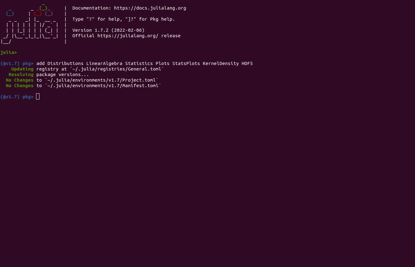
Once the julia language has been installed, some essential julia packages are required to be added that help simplify linear algebra and statistical calculations, and plotting. To add these packages via julia REPL, first enter the julia package manager by executing "]" command in the REPL. Then simply execute the following command to install all these packages at the same time.
add Distributions LinearAlgebra Statistics Plots StatsPlots KernelDensity HDF5
Also, see the image below for an example of the package installation process in julia REPL.
The samplers here execute a Markov Chain Monte Carlo (MCMC) algorithm (Gibbs) where samples for each parameter of interest are generated sequentially from their corresponding probability distributions (posterior). First, the sampler creates/initiates arrays to store all the samples, posterior values, and acceptance rates for proposed samples. Next, new samples are then iteratively proposed using proposal (normal) distributions for each parameter, to be accepted or rejected by the Metropolis-Hastings step if direct sampling is not available. If accepted, the proposed sample is stored in the arrays otherwise the previous sample is stored at the same MCMC iteraion.
The variance of the proposal distribution typically decides how often proposals are accepted/rejected. A larger covariance or movement away from the previous sample would lead to a larger change in likelihood/posterior values. Since the sampler prefers movement towards high probability regions, a larger movement towards low probability regions would lead to likely rejection of the sample compared to smaller movement.
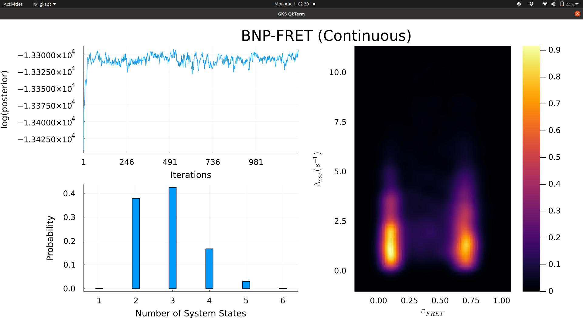
The collected samples can then be used to compute statistical quantities and plot probability distributions. The plotting function used by the sampler in this code allows monitoring of posterior values, most probable model for the molecule, and distributions over transition rates and FRET efficiencies.
As mentioned before, sampler prefers movement towards higher probability regions of the posterior distribution. This means that if parameters are initialized in low probability regions of the posterior, which is typically the case, the posterior would appear to increase initially for many iterations (hundreds to thousands depending on the complexity of the model). This initial period is called burn-in. After burn-in, convergence is achieved where the posterior would typically fluctuate around some mean/average value. The convergence typically indicates that the sampler has reached the maximum of the posterior distribution (the most probability region), that is, sampler generates most samples from higher probability region. In other words, given a large collection of samples, the probability density in a region of parameter space is proportional to the number of samples collected from that region.
All the samples collected during burn-in are usually ignored when computing statistical properties and presenting the final posterior distribution.
Each specialization of BNP-FRET (continuous or pulsed illumination) is organized in such a way that all the user input is accomplished via the "input_parameters.jl" file. It can be used to provide file names for experimental FRET data and sampler output, background rates for each detection channel, crosstalk probabilities, and plotting options. See the respective files for more details (they are well-commented). The functions involved in the both specializations of BNP-FRET and their respective outputs are briefly described below:
The functions used to perform all the computations are organized in a hierarchical structure. The file "sampler_continuous_illumination.jl" contains the main sampler. All the functions called in that file are written in the file "functions_layer_1.jl". Similarly, all the functions called in the file "functions_layer_1.jl" are in file "functions_layer_2.jl". Any new set of functions can be introduced by following the same heirarchical structure. A brief description of all the functions is given below in the sequence they are called:
-
get_FRET_data(): Used to obtain photon arrival data and corresponding detection channels from input files in HDF5 format. It can be easily modified if other file formats are desired.
-
sampler(): Used to generate samples for parameters of interest using Gibbs algorithm.
-
check_for_existing_mcmc_data(): Called by sampler() to searche for previously generate MCMC samples stored in HDF5 format files in the working directory.
-
initialize_params(): Called by sampler() to initialize all the parameters of interest to constitute the first set of MCMC samples.
-
get_log_likelihood(): Called by sampler() to computes the logarithm of the likelihood function for the FRET data.
get_generator(): Called by get_log_likelihood() to obtain the full generator matrix containing photophysical and biomolecular transition rates.
get_rho(): Called by get_log_likelihood() to obtain the initial probability vector associated with the generator matrix.
non_radiative_propagator: Called by get_log_likelihood() to compute propagators during periods when no photons are detected.
radiative_propagator: Called by get_log_likelihood() to compute propagators at photon arrival times.
-
get_log_prior_rates(): Called by sampler() to obtain logarithm of prior density at a parameter's value.
-
get_log_full_posterior(): Called by sampler() to get full joint posterior. Sums logarithms of likelihood and all the priors.
-
save_mcmc_data(): Called by sampler() to save output to files.
-
print_and_plotting(): Called by sampler() to print values on standard out (terminal/screen). It also generates plots (shown in the example below).
-
propose_params(): Called by sampler() in the for loop to propose new samples for each parameter that may or may not be accepted in the Metropolis-Hastings (MH) step.
An example of code output below shows the MCMC (Markov Chain Monte Carlo) iteration number (number of samples generated), number of active system states, labels for all the active loads, the excitation rate (related to laser power), rate matrix for the biomolecule of interest with FRET efficiencies on the diagonal instead of zeros, logarithm of the full joint posterior, and acceptance rates. We used smFRET data from experiments studying binding and unbinding of intrinsically disordered proteins (immobilized ACTR and freely-diffusing NCBD) in presence of 36 % ethylene glycol to generate this output.
https://www.pnas.org/doi/full/10.1073/pnas.1921617117
=================================================================

Iteration: 1217

n_system_states = 4

loads_active = [1, 3, 5, 6]

excitation rate (s^(-1)) = 4111.3703223987695

rate_matrix (s^(-1)) (diagonal elements show FRET efficiencies) =

4×4 Matrix{Float64}:
 0.0944715  0.650713    0.0648545  0.10982
 0.411844   0.709043    0.729846   1.80119
 2.97991    2.91667     0.487081   0.432123
 0.869362   0.00541285  0.700872   0.054417

log_full_posterior = -13304.721733757791

minimum, median, maximum acceptance rate = 60.72308956450287%  61.750205423171735%  88.82497945768283%

=================================================================
Furthemore, the sampler output can be visualized using the plotting options in the "input_parameters.jl" file. Visualization of the sampler output makes it easy to identify when the posterior converges and the most probable model (number of system states). Furthermore, it shows a bivariate distribution for FRET efficiencies and escape rates (sum of all the rates out of a state or in a rate matrix row). All the samples until the full joint posterior reaches convergence (maximum value) should be ignored. This initial period is also known as burn-in. For efficient exploration of the parameter space, tune the covariance values for the proposal distributions in such a way that the acceptance rates stay between 30 and 60% approximately.